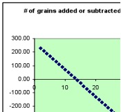
Defining Functions Iteratively – Variations on a Folk Tale There is a legend about the game of chess. When the creator of the game of chess showed his invention to the ruler of the country, the ruler was so pleased that he gave the inventor the right to name his prize for the invention. The man, who was very wise, asked the king this: that for the first square of the chess board, he would receive one grain of wheat (in some tellings, rice), two for the second one, four on the third one, and so forth, doubling the amount each time. The ruler, arithmetically unaware, quickly accepted the inventor's offer, even getting offended by his perceived notion that the inventor was asking for such a low price, and ordered the treasurer to count and hand over the wheat to the inventor.[1] The key to understanding this story and the astonishment of the ruler is the rule that was proposed to calculate the number of grains of wheat to be added each day – i.e. start with one grain of wheat on the first day and each day afterward add twice the number of grains of wheat that were added the day before. This rule generates an exponential growth of numbers of grains of wheat. The rule the inventor chose to determine the change in the number from square to square is an example of a different way of defining a function from that which is ordinarily used in algebra. The function is defined by an iterative procedure – we are told how many to start with and we are given a rule for calculating the change from each square to the next square. Defining functions iteratively is at the heart of that branch of applied mathematics that uses calculus to build models of complex phenomena in physics, chemistry, biology and economics, not to mention a wide variety of engineering fields. The story cited above describes an iterative procedure that leads to an exponential function. But the inventor in that story could have chosen other rules to determine how many grains of wheat to put down on the chessboard. The object of this paper is to examine other rules and in particular rules that lead to the generation of the functions most focused on in early algebra - linear, quadratic and absolute value functions. Defining Functions Iteratively Here are illustrations from a spreadsheet that explores these other rules for adding (or subtracting) grains. The simplest change rule is to start with some number of grains of wheat and add a fixed number of grains of wheat each day. Here is a spreadsheet that shows what happens when one starts with 100 grains and adds two grains each day.
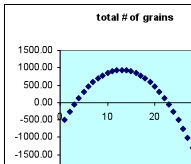
 If the same change is made each day, as in this case, then the total number of grains as a function of time will be a linear function of the number of days. By choosing the starting number you can control the vertical intercept. If you add a constant amount each day the total number of grains as a function of time will be a linear function with positive slope. If you subtract a constant number each day the total number of grains as a function of time will be a linear function with negative slope. A linear function has the property that if you evaluate a linear function at uniformly spaced points in its domain, the values of the function for adjacent points will differ by a constant value. This is exactly how we calculated the number of grains to add each day in this case. Suppose we choose a somewhat more complicated rule – suppose that each day we add a number of grains that is proportional to the number of days that have elapsed since the beginning of the procedure. For example, we might start with 100 grains on day 0 and then add 3 grains on day 1, 6 grains on day 2, 9 grains on day 3, etc. Here is a spreadsheet that shows what happens when we do that.
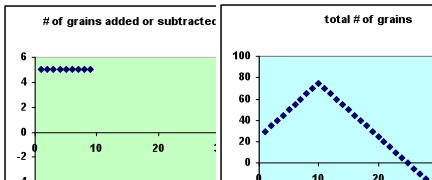
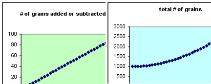 The total number of grains as a function of the number of days now looks very much like a quadratic function. Is it really a quadratic function and how can we tell? A quadratic function has the following property – if you evaluate a quadratic function at uniformly spaced points in its domain, the values of the function for adjacent points will differ by an amount that changes linearly. This is exactly how we calculated the number of grains to add each day in this case. Finally, let’s consider what kind of rule leads to the third family of functions widely used in early algebra – the absolute value function. Absolute value functions are made up of two sections each of which is linear but the two linear sections have slopes that can be written as m and – m. We have seen that the change = constant rule leads to a total number of grains function that is linear. Suppose we use amend that rule in this way – let the change from the start to some particular later day be say 5 grains/day and after that particular day –5 grains/day. Here is a spreadsheet of that rule.
 These sorts of rules can be
more general than the cases we have looked at in several ways.
Here is an example of a combined change rule [change = constant + multiple of day #] .
By now it should be clear
that the rules we have been examining seem to produce linear, quadratic and
absolute value functions for the total number of grains.
This way of defining functions is powerful for several reasons that we have not yet discussed.
The Relation between this Way & the Traditional way of Defining Functions Traditionally, two parameters are used to define a linear function. There parameters could be the slope and intercept with the vertical axis, the slope and intercept with the horizontal axis or the
two intercepts with the axes. After the two parameters are specified, values of the function for a given value of the variable can be calculated. Similarly, three parameters define a quadratic function. Traditionally the quadratic function is written in one of three standard forms: y = ax2 + bx + c (polynomial form)
y = a(x – r1)(x – r2) (root form)
y = a(x – h)2 + k (vertex form) After the three parameters are specified, values of the function for a given value of the variable can be calculated. The families of absolute value functions used in early algebra are all of the form F(x) = a|x + b| + c which also require specifying three parameters. How does this new way of producing linear, quadratic and absolute value functions correspond to what we have done earlier? The rule change = constant which produced a linear function for the total number of grains required us to specify two numbers, the number of grains to start with and the number to add or subtract each day. These parameters are quite different in nature from the ones that are used in the traditional definition of the linear function. The rule change = K x day # which produced a quadratic function for the total number of grains required us to specify two numbers, the number of grains to start with, and the multiple of the day number to add or subtract each day. Although only two parameters are needed to generate these quadratic functions, this rule can only produce quadratic functions whose graphs start out flat and either always increase or always decrease. Can you see why this is so? The rule change = constant + K x day # which produced a quadratic function for the total number of grains required us to specify three numbers, the number of grains to start with, a constant number to add or subtract each day and the multiple of the day number to add or subtract each day. Here too it will be noticed that these parameters are quite different in nature from the ones that are used in the traditional definition of the quadratic function. The rule change = constant up to a particular day combined with change = - constant after that day which produced an absolute value function for the total number of grains required us to specify three numbers, the number of grains to start with, the number to add or subtract each day in the beginning and the number of the day on which to switch from adding to subtracting (or vice versa). In order to help answer the question of the correspondence between the traditional way of defining these functions and the way we have done so here let’s introduce a somewhat less awkward notation. Suppose we call the total number of grains n days after we start Gn grains Then the first rule change = constant can be written Gn+1 grains = Gn grains + C grains/day x 1 day The second rule change = K x day # can be written Gn+1 grains = Gn grains + K grains/day x n days The third rule change = constant + K x day # can be written Gn+1 grains = Gn grains + C grains/day ´ 1 day + K grains/day x n days The fourth rule can be written in two parts: Gn+1 grains = Gn grains + C grains/day x 1 day, on days before day T Gn+1 grains = Gn grains – C grains/day x 1 day, on days after day T It would be good to write these rules even more generally. Clearly we can make such
rules for accumulating things other than grains of wheat – we can, for example,
accumulate grams of a liquid in a container that is filling or meters of
distance covered as we go on a trip. Instead of grains, therefore let us use
the symbol X for the amount of the quantity we are accumulating. Secondly, we need not restrict ourselves to an increment a day. We could increment our amts every second, or every minute, or every week, or every year. To indicate this let us call the time between increments ∆ t (read delta t). These changes lead to the following notation: The total amount at time t after we start can be written as G(X, t) Each of the rules we have studied can now be written in the form G(X, t + ∆ t) = G(X, t) + change where change stands for the amount added or subtracted each time period ∆ t . In their more general form our rules look like this: The first rule change = constant can be written G(X, t + ∆ t) = G(X, t) + C X / ∆ t x ∆ t The second rule change = K x day # can be written G(X, t + ∆ t) = G(X, t) + K X / ∆ t x t The third rule change = constant + K x day # can be written G(X, t + ∆ t) = G(X, t) + C X / ∆ t x ∆ t + K X / ∆ t x t The fourth rule can be written in two parts: G(X, t + ∆ t) = G(X, t) + C X / ∆ t x ∆ t , for t < T G(X, t + ∆ t) = G(X, t) – C X / ∆ t x ∆ t , for t > T The units of each term in these rules are the units of X. The units of the C and the K that appear in these rules are the units of X / ∆ t. Does ∆ t Matter? You might well ask why we bother to write the change as C grains/day x 1 day in the case of the first rule or K grains/day x n days in the second and third rules. Here’s why. Suppose we wanted to try these rules for a year – with a change of say 30 grains/day and 5 times the day number. That would make a very long table in the spreadsheet. Couldn’t we write the rules in the following way; first rule change = constant as Gn+1 grains = Gn grains + 210 grains/week x 1 week second rule change = K x day # as Gn+1 grains = Gn grains + 35 grains/week x n weeks third rule change = constant + K x day # as Gn+1 grains = Gn grains + 210 grains/week x 1 week + 35 grains/week x n weeks In that way we could find out how many grains we had at the end of a year in just 52 steps. Or if we wanted an even shorter table we could make our changes every month – in that case (for a 30 day month). In that case... the first rule change = constant becomes Gn+1 grains = Gn grains + 900 grains/month x 1 month the second rule change = K x day # becomes Gn+1 grains = Gn grains + 150 grains/month x n months the third rule change = constant + K x day # becomes Gn+1 grains = Gn grains + 900 grains/month x 1 month + 150 grains/month x n months which would give us a number of grains at the end of the year in just 12 steps. Aren’t all the following quantities all equivalent to 30 grains/day? 210 grains/week, 900 grains/month, 30/24 grains/hour, 30/(24 x 60) grains/minute, etc Yes, of course – BUT! the way we are using these quantities in our rules for accumulating grains (or in general amounts of anything) means that the size of the change may depend on when the change is made. For example, let’s consider the following case: Start from 0 grains and add 5 grains a day for 60 days or add 150 grains a month for 2 months. Using the change = constant rule, both of these cases will result in 300 grains accumulated at the end of 60 days or 2 months. On the other hand suppose we consider starting from 0 grains and adding K = 5 grains/day x day # for 60 days or adding K = 150 grains/month x month # for 2 month using the change = K x time period # rule. Using this rule, if we add 5 grains/day for 60 days we get an accumulation of 9,150 grains. Adding 150 grains a month results in accumulation of 450 grains! Briefly stated our rule for generating linear accumulation functions does not depend on the size of the time increment. Our rules for generating quadratic functions do depend on the size of the time step. These rules will always generate quadratic functions but different time steps will lead to different quadratic functions. As the time steps become shorter and shorter, the quadratic accumulation functions generated by our rules get closer and closer to one another. The calculus provides an explanation for why this is the case. Appendix What
happens in the original tale? In the
original tale the number of grains added is twice the number added the day
before. This change rule is
Gn+1 = 2 x [Gn – Gn-1] with G0 = 1
It is easy to see that Gn = 2n x G0. On the 64th day the number of accumulated grains would be 18,446,744,073,709,551,615 [1] From Wikipedia. The story continues…However, when the treasurer took more than a week to calculate the amount of wheat, the ruler asked him for a reason for his tardiness. The treasurer then gave him the result of the calculation, and explained that it would be impossible to give the inventor the reward. The ruler then, to get back at the inventor who tried to outsmart him, told the inventor that in order for him to receive his reward, he was to count every single grain that was given to him, in order to make sure that the ruler was not stealing from him. - Wikipedia
|