[to explore a collection of applets that illustrate the ideas in this paper please go to Formulating Measures]

Formulating Measures:

toward modeling in the K-12 science and mathematics curriculum

On Measures and Models

In science and mathematics education, all too often problems involve selecting an already formulated model that describes/explains the phenomena in question and then selecting the “correct” relation among relevant aspects of a situation and quantitatively evaluating it.

If however, science and mathematics education is about teaching people how to build and use ever more effective models of phenomena should we not focus that education on formulating the relations and the elements that are related by these models?

We do focus on such relations embodied in our models of how the distance traveled by a falling body depends on its initial velocity and the height from which it is released or how energy is transformed from energy of motion into energy of configuration and back in systems that oscillate.

But the quantities that are the elements that are related by these relationships, kinetic energy, potential energy, velocity, acceleration, are all measures that we tell our students are worth attending to. Indeed they are. But our students have not had a hand in formulating these measures that are the elements linked by the models we build and use.

It is important to stress that measures are not models – rather, they are the elements of models. In the sciences, models describe how measures are related to one another, and perhaps most often, how they vary in time and/or how they vary in space.

It is centrally important to the practice of many natural and social science disciplines to go through the exercise of forming measures[1] of quantities of interest. Indeed it may be said that the formulation of measures is an important first step in the act of modeling – with the measure itself serving as the heart of a structural model, or the time dependence of the measure as the core of a functional model[2].

Geographers[3] studying spatial segregation patterns, computer scientists[4] studying the evolution of biological complexity, biochemists[5] trying to establish similarity of metabolic pathways, reading specialists[6] studying dyslexia in children and public health physicians[7] studying stress in neighborhoods to name but a few examples of measures devised by scientists working in diverse disciplines.

The essence of a measure is the fact that it can be ordered. Humans seem to have an insatiable desire to rank order. Consider the ubiquitous “10 most…” and “10 best…” lists that are found in popular magazines. The annual rank ordering by news weeklies of US colleges and universities is anxiously awaited each year by admissions offices throughout the country.

Sometimes we seek to order quantities that are directly accessible to the senses such as heights and weights. The rank ordering of such quantities is relatively straightforward, although it may require the introduction of instruments to refine or extend our senses. Sometimes, however, we seek to order quantities that are clearly dependent on several, or even many, contributing factors such as cost of living or the efficiency of an automobile.

It is important when ordering such complex quantities that the bases for the orderings be made explicit and public. This may permit one to say that in the ordering A, B, C whether B is closer to A than it is to C and if so, by how much. When this happens it is fair to say that we have devised a measure of the scale along which A, B, and C are arrayed.

This paper is a plea for a new kind of task – one that asks students to formulate measures of their own – as a step in the direction of understanding how models are made.

What are measures?

Measures are either directly observed continuous or discrete quantities or quantities computed from observed continuous or discrete quantities

We need to sharpen the distinction between assigning magnitude to discrete quantities and assigning magnitude to continuous quantities. We note that it is possible to use the word one with count nouns but not with mass nouns.  Thus, one may say, one apple or one person but not one clay or one water. Indeed, we may use any integer as an adjective with count nouns. In attaching a magnitude to a count noun, we have to make a judgment that takes all the attributes of the referent object into account and which results in a single yes-or-no decision as to whether the object we are considering does or does not belong to the class of things to which we are assigning number.  Thus, before being able to say one apple, we must take into account the size, color, shape, weight, etc. of the object before us, and conclude, yea or nay, does this object, with all the values of all its attributes, satisfy our requirements for being an apple. Similarly, the problem of counting all the chairs in a house requires that we make decisions about objects that may be as disparate as easy chairs, stools, chaise lounges and probably even step ladders.  For each object considered, color, form, size and materials need to be taken into account and a single dichotomous decision arrived at, i.e. is the object in question a chair?  It goes without saying that the only sort of number that can result from the act of counting is an integer.

On the other hand, in the case of mass nouns, we can introduce adjectival quantity only after we have singled out the attribute of the referent object that we wish to quantify.  We say, for example, three hundred grams of clay.  In so doing we ignore the shape of the clay and its color and focus solely on its weight (more properly its mass, in this case).  Because of these considerations, it is clear that the result of assigning size to some attribute of a mass noun, an act we normally call measuring, necessarily results in a non-negative rational number.[8]

Perceptually available (simple) measures

Humans come equipped with “hardware” to assign at least relative size to certain sorts of measures. These include:

Counts, Lengths, Areas, Times, Weights, Speed(?)

Composite measures - Qualitative relations among simple measures      

We can form combinations of perceptually available measures in order to generate more complex measures that may be more informative in more complex situations. Clearly the simplest form of combination is one that combines two simple measures.

We consider first a form of combination that leads to Direct Variation. We refer to such combinations as Product Measures.

A Product Measure is composite measure C that depends on two component measures A and B such that

if A increases then C increases - more A implies more C

if B increases then C increases - more B implies more C

Assume we have a collection of objects (say, pickup truck, fast pitched baseball, car, motorcycle, bicycle, etc.) that are moving. Most people would be willing to agree that there is some property of a moving pickup truck that is usually “larger” than that of a moving bicycle. Suppose, for the moment, we call this property “oomph”

Is there some way we can pin down what such a property called “oomph” might be? More to the point, is there some way we can say whether the “oomph” of some other moving object is closer to the “oomph” of the pickup truck than it is to the “oomph” of the bicycle? And if so, how much closer?

More generally, if we have a bunch of different moving objects, can we find a way to order them according to the “oomph” property – from the one with the “largest” to the one with the “smallest”?

First thoughts would suggest that the relevant properties of the moving objects that we want to pay attention to are how heavy they are and how fast they are moving. Each of the moving objects has both a mass and a speed.

Assuming we have the proper instruments for measuring speed and mass, we could measure both the speed and the mass for each of the moving objects. If we do so, we will quickly discover that our mystery property, “oomph”, cannot be mass and it cannot be speed. A baseball, which is clearly less massive than a car, can be much harder to stop that a slowly rolling car. By the same token, even a very slowly rolling locomotive can be much harder to stop than a fast moving car [a fact that can be attested to by many drivers injured in attempting to beat a train across a grade crossing].

Clearly, any measure of this “oomph” property has to take both speed and mass into account.

Let us put on hold for the moment making such a measure quantitative and turn to its logical complement -  a form of combination that leads to Inverse Variation. We refer to such combinations as Quotient Measures.

A Quotient Measure is a composite measure C that depends on two component measures A and B such that

if A increases then C increases - more A implies more C

if B increases then C decreases - more B implies less C

If we have a collection of pieces of aluminum (say, an aluminum saucepan, a door hinge, a machine screw) and a collection of pieces of pine (say, a cutting board, a small jewelry box, a chess piece) and a collection of pieces of polystyrene (say, several different food containers) most people would be willing to agree that there is some property of aluminum that is “larger” than that of pine. Suppose, for the moment, we call this property “oomph”

Is there some way we can pin down what such a property called “oomph” might be? More to the point, is there some way we can say whether the “oomph” of some third material like polystyrene is closer to the “oomph” of aluminum than it is to the “oomph” of pine? And if so, how much closer?

More generally, if we have a bunch of different materials, can we find a way to order them according to the “oomph” property – from the one with the “largest” to the one with the “smallest”?

First thoughts would suggest that the relevant property of the aluminum pieces, the pine pieces and the polystyrene pieces that we want to pay attention to is how “big” they are. But by “big” we might mean their physical size (volume – amount of space they take up) or we might mean their weight (or their mass). Clearly each piece of aluminum, pine and polystyrene has both a volume and a mass.

Composite Measures - Quantitative Relations among simple measures

In many situations we go beyond the qualitative variation considered in the previous section. Consider, for example a product measure such as momentum.

Returning to the qualitative attempt at formulating a measure that captures a direct variation – the problem of stopping a moving object

In order to formulate a measure of “oomph” we could try to “add” measures of speed and mass. However, doing so leads to the unfortunate result that a body could have “oomph” even if it were standing still. Also, this kind of measure of “oomph” leads to the conclusion that even a particle with no mass can have “oomph” 

A more successful measure of “oomph” would be a product of mass and speed. This sort of measure avoids the difficulties that the previous proposed measure had. With this measure a moving object has no “oomph” if it is standing still. Moreover, even at a fixed speed, the smaller the mass of the moving object, the smaller its “oomph”.

This measure of how difficult it might be to stop a moving object is normally not called “oomph” but is called momentum.

Here, for example is a task that requires the formation of a product measure – one that is well-known to be difficult for middle school, and even upper elementary students.

The measure in question in this example is “Size of Available Menu”

Lest one think that formulating product measures is a problem only for young students consider the following example of a measure of efficiency for different aircraft types.

• area [~length²]
• volume [~length³]
• combinations[~counts•counts]
• work [~force•length or ~ mass•length²/time²]
• momentum [~mass•velocity or ~mass•length/time]
• passenger-miles [~counts•length]
• kilowatt-hours [~energy/time•time or ~mass•length²/time²]
• flux [~(mass/distance)•(distance/time){1D}, ~(mass/volume)•(volume/time){3D}]

Such Product Measures are almost always extensive quantities and are rarely (if ever) dimensionless.

Returning to the qualitative attempt at formulating a measure – one that captures an inverse variation – the problem of characterizing a material (rather than an object made of that material).

Assuming we have the proper instruments for measuring volume and mass, we could measure both the volume and the mass for each of the pieces of aluminum, pine and polystyrene. If we do so, we will quickly discover that our mystery property, “oomph”, cannot be mass and it cannot be volume. We can find some pieces of pine with more mass than pieces of aluminum and some pieces of pine with less mass than pieces of aluminum.

Here are data from the measurement of masses and volumes and a scatter plot of those data.

A scatter plot of these data looks like this: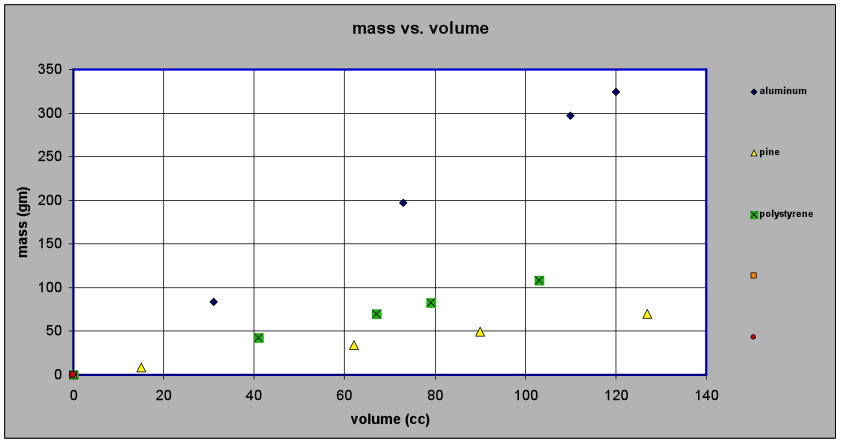

Normally, we present the concept of density somewhere in middle school as the ratio of mass to volume. If however, we proceed from the data, we see that doing that constitutes a leap! We have a finite number of data points – the assertion that

Density = mass / volume

For all non-negative values of mass and volume is an assertion of a model. It is a predictive model allowing us to predict the magnitude of the mass of a piece of material whose volume we have measured but whose mass we have not measured. Similarly, the model allows us to predict the value of the volume of a piece of material whose mass we have measured but whose volume we have not measured.

Quotient Measures such as density are almost always intensive quantities and are  sometimes dimensionless.

There is a caveat that must be expressed here about this model of density. This is fundamentally a formulation of a macroscopic model of density.  It depends on the assumption that seems to work perfectly well in our macroscopic world . i.e. that when two masses are put together their combined mass is the some of their masses and that when two volumes are put together their combined volume is the sum of their volumes.

The reader is invited to consider whether these assumptions are true on a microscopic scale or on a galactic scale.

Some perceptually based Quotient measures

As a way of ramping up to the introduction of measure formulating tasks into the curriculum we describe here a series of such tasks that are largely based on visual perception and that require little or no external or prior knowledge to begin the task. The full tasks are to be found on the challenge section of this website.

"Square-ness" is a formulating measures task that demands virtually no prior knowledge to begin. Nonetheless it presents a nice opportunity to have students devise measures – several perfectly reasonable ones are likely to arise in discussion – and to discuss their relative merits.

Students are shown a collection of rectangles of varying sizes and aspect ratios and presented with the following questions -

• 1.  Which of the rectangles is the “squarest”? 
• 2.  Arrange the rectangles in order of “square-ness” from most to least square. 
• 3.  Devise a measure of “square-ness,” expressed algebraically, that allows you to order any collection of rectangles in order of “squareness.” 
• 4.  Devise a second measure of “square-ness” and discuss the advantages and disadvantages of each of your measures.       

An interesting extension of this task is to consider the ordering a set of parallelograms in order of “Square-ness”

Densities can be linear densities as in the case of traffic flow. Densities can be area densities as in the illustrative example. Densities can be volume densities as in the classic case of mass density.

Other volume densities that we have found students have much difficulties with include electric charge density and energy density in energy storage media such as batteries or capacitors as well as energy density in propagating electromagnetic waves.

Additive measures

Are there measures that are more complex than product measures and quotient measures that play a role in K-12 education?

Here is an example:

Additive Measures of the form

c₁A₁ + c₂A₂ + … + c_nA_n

 where the set {A_i} denotes the set of attributes that are deemed to be important for the composition of the measure and the set of coefficients {c_i} are used to make the measure dimensionally coherent and also to express the relative importance of the different attributes in composing the measure.

In general, measures in the social sciences have this sort of structure. Probably the best known example is Gross National Product (GNP) which is a linear combination of a large number of indicators with suitable coefficients so that the combined measure is in dollars.

Is The Measure “Good Enough”?

Choosing a measure to characterize the state of a system is an exercise in deciding what features of the system one wants to include in ones characterization and what features are sufficiently unimportant for the purpose at hand that they may be neglected, at least at first.

For example, a measure of density may not, at first, contain any reference to temperature. A measure like momentum may contain at first a reference only to the speed of the center of mass of a body and not refer to the distribution of mass and velocity within the body.

Thus the process of formulating a measure as a first step on the road to modeling is of necessity a tentative one. Ultimately, the question of “is the measure good enough” can only be answered by listening to the fugue of the predictions of the model formulated with this measure and the purpose for which the model has been formulated.

From Measures to Models

Measures that are models & measures that are not models

Are measures models? That depends. In my view an essential property of a model is its ability to predict the value of a measure in an as yet untried instance.

In the case of density discussed above, we designed a measure (and called it density) based on data collected from a variety of objects that were fashioned from a variety of materials.

Can we predict the value of the density measure for an object whose mass and volume we have not previously measured? Under limited circumstances the answer is yes. If the material is one with which we have worked before then using our rule for how mass and volume are related for the material in question -

if we measure the mass we can predict the volume

if we measure the volume we can predict the mass

if we measure the mass and the volume we can calculate the ratio of mass to volume[9]

On the other hand, if we have not worked with the material before we cannot make such predictions.

In contrast, consider “-ness” measures such as “square-ness”. Despite the fact that the task was presented with a finite number of rectangles we did not infer a rule for quantifying “square-ness” from these few rectangles. What we did was to assert a rule for calculating the value of the measure we defined as “square-ness”. This is in contrast to the density case where we were dealing with real objects made from real materials and we were obliged to devise our rule from limited data. In the case of rectangles, by asserting our rule for calculating the measure we took all rectangles into account in formulating our measure. As a result there are no as yet untried instances. Thus from my perspective, “square-ness” is not a model – it is simply a measure.

In the case of our measure of “difficulty of stopping a moving object” we have a related situation. We have asserted that the value of the momentum of any moving object can be calculated from knowing the mass and the speed of that object. There are no as yet untried instances. Momentum, by itself, is not a model – it is a measure.

It took an Isaac Newton to assert a model – i.e. that the time rate of change of this measure called momentum is equal to the applied force.

Getting from Measures to Models

The centrality of “as yet untried instances” to this discussion is by now evident. It is a manifestation of the need for models to be falsifiable[10]. A measure whose value may always be calculated from its definition is thus clearly not a model.

Does this mean that measures are not germane to a discussion of models? Not at all. Measures are the constructs we need to formulate in order to build models. A model in physics, for example, may predict how a measure like momentum will change with time. A model in chemistry may predict how a measure like concentration of a species might change with time. A model in economics might predict how a measure like gross national product might change with time. A model in environmental science might predict how a measure like average global temperature might change with time.

Measures can vary with parameters other than time – e.g., measures such as density and pressure in gases can vary with temperature. The essential point is that in order to have a model we must be able to predict the values of a measure that we are interested in instances that did not enter into the formulation of that measure. For example, in the case of density, we found our empirical data for the case of aluminum to be well described by

M (mass in grams) = 2.73 grams/cc x V (volume in cc)

The assertion that this relationship is valid beyond the data points that were used to construct this description is a model for aluminum. The assertion that for any homogenous material the mass of an object is proportional to its volume is a generalization of this model to all homogeneous materials. The further assertion that for any homogeneous material the constant of proportionality is inversely proportional to the temperature is a still further generalization of the model.

Ideally, one would like to predict how the values of the measure one formulates might vary with time or temperature or some other parameter(s) of interest. However, we may not understand the underlying science well enough to be able to make quantitative predictions. We may, however, have a qualitative understanding of underlying mechanisms that is good enough for us to say the value of our measure will increase or decrease with time or temperature. Such semi-quantitative models have been the subject of some considerable investigation[11],[12]

Agent-based models – from local interactions to global measures of complex behavior

Up to this point we have discussed measures that for the most part can be thought of as macrosopic measures – measures that are characteristic of an entire system and do not vary from one part of the system to another. Needless to say, this is not always the case. Density can depend on position as NASA discovered when it first orbited a satellite around the moon and found that the mass of the moon was not homogeneously distributed.

The explosive growth of computational power that has become increasingly widespread in the past decades has enabled us to approach the problem of modeling phenomena of all sorts in a fashion that differs greatly from that which has been discussed so far. Such models are called “agent-based” models and are particularly valuable in modeling systems whose properties of interest may vary from place to place. Agent-based models are built on the assumption that phenomena can be simulated by considering a large number of agents that interact with one another in space and time via interactions that can be simply stated and whose consequences may be computed simply. Although the possibility of such models was first described in the 1940s it was not until the widespread availability of computers that it became realistic to model phenomena in this fashion.

Here is a quote from a description of agent-based models[13]:

The situatedness of the agents and their responsive, purposeful behavior are encoded in algorithmic form in computer programs. The modeling process is best described as inductive. The modeler makes those assumptions thought most relevant to the situation at hand and then watches phenomena emerge from the agents' interactions. Sometimes that result is an equilibrium. Sometimes it is an emergent pattern. Sometimes, alas, it is an unintelligible mangle.

Here is an example drawn from an agent-based model of fish and shark populations[14] in a rectangular grid:

The upper part of the illustration shows the location of fish and sharks at a particular instant in the evolution of the system. The lower part of the illustration shows two graphs, one of the fish population as a function of time and the other the shark population as a function of time.

Despite the fact that the rules governing the behavior of individual fish and individual sharks are quite simple we see that quite complex oscillatory behavior can emerge when the model is run. Here is a short summary of the rules that govern the interactions of the fish and sharks with one another and with the environment[15].

The program is dependent upon five parameters, plus the size of the rectangular grid. The first parameter is the number of fish, the prey. A fish swims at random to one of the four horizontally or vertically adjacent spaces on the grid, if it is unoccupied. … The second parameter is the fish breed time. If a fish survives this number of cycles and an open space is available, a new fish is bred. The third parameter is the number of sharks, the predators. A shark eats a fish in an adjacent space on the grid. A shark swims to an open space if there is no adjacent fish. The fourth parameter is the shark starve time. If a shark finds no fish for this number of cycles, it dies. The final parameter is the shark breed time. A shark breeds in the same way as a fish.

If the number of sharks is very small, the fish population will increase quickly and the shark population will soon follow because they find plenty of food. Eventually the fish will become overcrowded and overwhelmed by the large shark population and the fish population will crash. Depending upon the quantity and distribution of sharks at the beginning of the crash, the fish may disappear entirely, the sharks may become isolated and disappear or catastrophe may be narrowly averted.

I cite this example in some detail to illustrate the fact that the statement of the individual fish and shark behaviors is the starting point of this model. The - as yet unexamined – entities in this model are the global measures[16] that emerge only after the individual fish and shark behaviors are allowed to develop. This is in contrast to the kind of model discussed earlier in which measures are formulated ab initio and then their time or other parametric behaviors are predicted.

Some implications for K-12 science and mathematics

The word “model” is widely used and, in my opinion, widely misused. By introducing the distinction between measures and models, as well as parsing the nature of simple and composite measures, it is my hope that explicit attention can be paid in K-12 science and mathematics classes to the formulation of measures. This in itself is a worthy effort that deserves attention as is apparent from even a brief consideration of some of the Balanced Assessment “–ness” tasks described above.

Moreover, separating the task of formulating a measure from that of formulating a model that uses that measure focuses attention on the distinction between the measure construct and the model construct. This is likely to result in a better understanding on the part of teachers and students of the differences and similarities between mathematics and science. But that is the subject of another discussion!

 Judah L. Schwartz

mathMINDhabits by Judah L. Schwartz is licensed under a Creative Commons Attribution-NonCommercial 4.0 International License.